How to Use the VLOOKUP Function in Excel

If you prefer video, check out the youtube tutorial

Download the file to follow along: Download

What is VLOOKUP?

VLOOKUP, short for "Vertical Lookup," is one of the most popular Excel functions for data analysis. It allows you to search for a value in one column and return a corresponding value from another column. This is especially useful when working with large spreadsheets, like matching employee IDs to names or linking countries to their capitals.

Let’s imagine you have two tables:

1. A list of countries and their capitals.
2. Another list of countries but without the capitals.

Instead of manually finding the capital for each country, VLOOKUP can do this for you automatically.

How to Use the VLOOKUP Formula

Here’s a quick overview of how to use the VLOOKUP formula in Excel:

Step-by-Step Guide:

Don't forget to download the file to follow along: Download

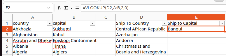
1. Start the formula: In cell E2 type =VLOOKUP( to begin.
2. Lookup value: The first argument is the value you want to search for. Click on the cell with that value (e.g., D2 for the country name).
3. Table array: Next, define the range of cells that contains both the lookup value (country) and the value you want returned (capital). Start by clicking on column A's header and hold the click and drag it across to column B. The first column you click should be the one that contains the field you're searching for (in this case Country). Then you want to make sure you drag the mouse to the column that contains the value you want to return (in this case Capitol).
4. Column index number: Specify which column the value you want to return is in (e.g., the third column for the capital). In this example it is 2.
5. Exact or approximate match: End with FALSE if you want an exact match, or TRUE for an approximate match. Honestly just use FALSE, I've never once needed to use TRUE.

=VLOOKUP(D2, $A:$B, 2, FALSE)

In this example:

• D2 is the lookup value (country name).
• $A:$B is the table array (the range where countries and capitals are listed).
• 2 is the column index number, meaning the second column (capitals).
• FALSE ensures an exact match.

Common VLOOKUP Mistakes

While VLOOKUP is powerful, there are some common mistakes to avoid:

• Incorrect range references: Make sure to use dollar signs ($) to lock your range.
• Wrong column index: Ensure the correct column number is specified for the value you want to return.
• Not using exact match: Always specify FALSE for an exact match, unless you want an approximate result.

Conclusion

The VLOOKUP function is an essential tool for data analysis in Excel. By using it, you can quickly find and reference values from large datasets, saving you hours of work. However, it’s important to understand the common mistakes and limitations of the function. For more complex scenarios, you may want to explore alternatives like INDEX MATCH or newer functions such as XLOOKUP.

If you want to see VLOOKUP in action, check out the video tutorial linked below where I demonstrate step-by-step how to use VLOOKUP efficiently. vlookup tutorial